CMEnt End-to-End Example
CMEnt Package
2026-06-11
Source:vignettes/cment_example.Rmd
cment_example.RmdGoal
This notebook showcases all CMEnt capabilities, including DMR scoring, motif extraction, motif-based DMR interactions, and visualizations.
Setup
suppressPackageStartupMessages({
    library(CMEnt)
    library(GenomicRanges)
    library(ggplot2)
})

genome <- "hg19"
Load Example Inputs
# loadExampleInputData fetches example resources from DMRsegaldata via
# ExperimentHub and assigns them into the current environment.
loadExampleInputDataChr5And11("beta")
loadExampleInputDataChr5And11("pheno")
loadExampleInputDataChr5And11("array_type")
# DMPs are produced from minfi, and have the form of a dataframe
loadExampleInputDataChr5And11("dmps")## Beta matrix dimensions: 43542 sites x 20 samples## Phenotype data dimensions: 20 samples x 3 columns## Array type: 450K## Number of DMPs (seeds): 23538## Head of phenotype data:## Sample_Group Age Gender
## T1 cancer 65 m
## T2 cancer 48 m
## T3 cancer 75 m
## T4 cancer 70 f
## T5 cancer 55 m
## T6 cancer 73 m## Head of DMPs:## intercept pval f qval pval_adj
## cg07461370 2.000713 1.792909e-03 -1.8944789 1.248781e-03 4.992027e-03
## cg04815577 1.866972 3.266108e-03 -2.4763589 2.074106e-03 8.291275e-03
## cg05648010 -1.263073 6.254793e-06 3.7266733 1.242563e-05 4.967167e-05
## cg22807585 -1.029384 3.612295e-04 -0.3214461 3.277151e-04 1.310047e-03
## cg26274580 -2.186916 1.993233e-02 -4.1934979 9.630916e-03 3.849976e-02
## cg25392700 -0.965860 1.313401e-02 -3.8039704 6.750557e-03 2.698547e-02
# The beta handler is used to retrieve beta values for the DMRs and their seeds, and to perform optional SVM-based scoring of the DMRs.
# It is better to initialize it once and reuse it, as it performs some pre-processing steps that are common across the DMRs.
# The beta handler can be supplied as the `beta` argument for the DMR calling and scoring functions, to avoid redundant initialization.
beta_handler <- getBetaHandler(beta, array = array_type, genome = genome)
DMR Assembly from Seeds
The buildDMRs function is used to build DMRs from the
provided seeds, which in this case are the DMPs. The function performs a
correlation-based expansion of the regions around the seeds, considering
both statistical significance and biological relevance of methylation
changes. To keep the vignette fast and reproducible during package
checks, we load a bundled example result generated with this workflow.
The resulting DMRs are stored in a GRanges object, which includes
metadata columns for the number of seeds and sites in each DMR,
delta-beta between sample groups, and DMR-level
pval/qval when seed p-values were supplied.
The number of DMRs found is reported.
pheno[, "case_control"] <- pheno$Sample_Group == "cancer"
dmrs <- readRDS(system.file("extdata", "example_outputChr5And11.rds", package = "CMEnt"))
cat(sprintf("DMRs found: %d\n", length(dmrs)))
## DMRs found: 2130## DMRs metadata columns: id, start_seed, end_seed, start_seed_pos, end_seed_pos, seeds_num, stop_connection_reason, connection_corr_pval, seeds, start_site, end_site, upstream_expansion_stop_reason, upstream_sites, upstream_expansion_length, downstream_expansion_stop_reason, downstream_sites, downstream_expansion_length, merged_dmrs_num, sites, supporting_sites_num, sites_num, sites_num_bg, seeds_num_adj, cases_beta, controls_beta, delta_beta, cases_beta_sd, controls_beta_sd, cases_beta_min, cases_beta_max, controls_beta_min, controls_beta_max, sites_cases_beta, sites_controls_beta, sites_delta_beta, sites_cases_beta_sd, sites_controls_beta_sd, sites_cases_beta_min, sites_cases_beta_max, sites_controls_beta_min, sites_controls_beta_max, in_promoter_of, in_gene_body_of, score, cv_accuracy, score_smoothed, segment_id, segment_slope, block_id, pwm, consensus_seq
cat(sprintf("DMRs genomic range example: %s\n", paste0(seqnames(dmrs)[1], ":", start(dmrs)[1], "-", end(dmrs)[1])))## DMRs genomic range example: chr11:192141-193016DMR Summary
DMRs are primarily summarized by genomic support, DMR-level
pval/qval when available, and methylation
effect size. The optional SVM-derived score and
cv_accuracy columns are complementary measures of how well
the DMR methylation pattern discriminates sample groups. In addition,
score trajectories are smoothed per chromosome and segmented, enabling
assignment of localized block IDs that capture saddle-like peaks in
Manhattan plots.
dmr_meta <- as.data.frame(mcols(dmrs))
summary_tbl <- data.frame(
    chr = as.character(seqnames(dmrs)),
    start = start(dmrs),
    end = end(dmrs),
    width = width(dmrs),
    seeds_num = mcols(dmrs)$seeds_num,
    sites_num = mcols(dmrs)$sites_num,
    delta_beta = round(mcols(dmrs)$delta_beta, 4),
    pval = if ("pval" %in% colnames(dmr_meta)) signif(dmr_meta$pval, 3) else NA_real_,
    qval = if ("qval" %in% colnames(dmr_meta)) signif(dmr_meta$qval, 3) else NA_real_,
    score = if ("score" %in% colnames(dmr_meta)) round(dmr_meta$score, 4) else NA_real_,
    cv_accuracy = if ("cv_accuracy" %in% colnames(dmr_meta)) round(dmr_meta$cv_accuracy, 4) else NA_real_,
    block_id = if ("block_id" %in% colnames(dmr_meta)) dmr_meta$block_id else NA_character_
)
if (any(is.finite(summary_tbl$qval))) {
    summary_tbl <- summary_tbl[order(summary_tbl$qval, -abs(summary_tbl$delta_beta), -summary_tbl$score, na.last = TRUE), ]
} else {
    summary_tbl <- summary_tbl[order(-abs(summary_tbl$delta_beta), -summary_tbl$score, na.last = TRUE), ]
}
knitr::kable(head(summary_tbl, 5), caption = "Top 5 DMRs by statistical evidence/effect size, with SVM score as a complementary measure")| chr | start | end | width | seeds_num | sites_num | delta_beta | pval | qval | score | cv_accuracy | block_id | |
|---|---|---|---|---|---|---|---|---|---|---|---|---|
| 1281 | chr5 | 1594676 | 1594733 | 58 | 4 | 4 | -0.5401 | NA | NA | 0.5634 | 0.75 | NA |
| 1280 | chr5 | 1555791 | 1556885 | 1095 | 3 | 5 | -0.4714 | NA | NA | 0.6938 | 1.00 | chr5_block8 |
| 53 | chr11 | 849800 | 850952 | 1153 | 2 | 3 | 0.4479 | NA | NA | 0.7209 | 1.00 | chr11_block4 |
| 654 | chr11 | 65374663 | 65375067 | 405 | 2 | 4 | 0.4152 | NA | NA | 0.7284 | 1.00 | chr11_block18 |
| 1470 | chr5 | 53751272 | 53751493 | 222 | 3 | 3 | 0.4106 | NA | NA | 0.7050 | 0.95 | NA |
Motif Discovery
Based on the seeds of the DMRs, motifs are extracted using the
extractDMRMotifs function (called by default when
buildDMRs is used). The function retrieves the sequences
around the seeds, applies a flank size of 5 bp, and identifies consensus
sequences. The number of DMRs with extracted motifs and the number of
unique motif consensus sequences are reported.
n_motif_consensus <- sum(!is.na(mcols(dmrs)$consensus_seq))
n_unique_motif_consensus <- length(unique(stats::na.omit(mcols(dmrs)$consensus_seq)))
cat(sprintf("Motifs extracted for %d/%d DMRs.\n", n_motif_consensus, length(dmrs)))
## Motifs extracted for 2130/2130 DMRs.## Unique motif consensus sequences: 2104Motif-Based DMR Interactions
Once motifs are extracted, the computeDMRsInteraction
function can be used to identify “interactions” between DMRs based on
motif similarity. The rationale is that DMRs with similar motifs may be
co-regulated or functionally related, even if they are not in close
genomic proximity. The function computes pairwise similarities between
the PWMs of the extracted motifs, excluding the center site positions,
corrects for microarray design biases, applies a minimum similarity
threshold of 0.8, and identifies connected components of interacting
DMRs. The resulting components are annotated with JASPAR motifs if
available. The number of interactions, components, and the size of the
largest component are reported. Additionally, the number of components
with JASPAR annotation is provided.
query_with_jaspar <- requireNamespace("JASPAR2024", quietly = TRUE)
interaction_results <- computeDMRsInteraction(
    dmrs = dmrs,
    genome = genome,
    array = array_type,
    min_similarity = 0.8,
    motif_site_flank_size = 5,
    min_component_size = 2,
    query_components_with_jaspar = query_with_jaspar
)
interaction_tbl <- interaction_results$interactions
component_tbl <- interaction_results$components
dmrs <- interaction_results$dmrs # The input DMRs are returned with additional metadata columns for the interactions and components.

cat(sprintf("Interactions found: %d\n", nrow(interaction_tbl)))
## Interactions found: 11## Components found: 11
if (nrow(component_tbl) > 0) {
    largest_component <- max(component_tbl$size, na.rm = TRUE)
    cat(
        sprintf(
            "Largest component size: %d / %d DMRs (%.2f%%)\n",
            largest_component, length(dmrs), 100 * largest_component / length(dmrs)
        )
    )
}
## Largest component size: 2 / 2130 DMRs (0.09%)
annotated_components_m <- !is.na(component_tbl$jaspar_names) & nzchar(component_tbl$jaspar_names)
annotated_components <- sum(annotated_components_m)
cat(sprintf("Components with JASPAR annotation: %d / %d\n", annotated_components, nrow(component_tbl)))
## Components with JASPAR annotation: 0 / 11
if (nrow(interaction_tbl) > 5) {
    knitr::kable(
        head(interaction_tbl[order(-interaction_tbl$sim), ], 5),
        caption = "Top 5 motif-similarity DMR interactions"
    )
}| index1 | chr1 | start1 | end1 | index2 | chr2 | start2 | end2 | sim | component_id | |
|---|---|---|---|---|---|---|---|---|---|---|
| 1 | 2018 | chr5 | 174905402 | 174905420 | 156 | chr11 | 2465491 | 2466655 | 0.8732051 | 1 |
| 3 | 163 | chr11 | 2593960 | 2594153 | 410 | chr11 | 43963820 | 43965126 | 0.8309401 | 2 |
| 6 | 1920 | chr5 | 153569823 | 153570512 | 1562 | chr5 | 76935080 | 76936793 | 0.8309401 | 9 |
| 4 | 786 | chr11 | 69589122 | 69590580 | 733 | chr11 | 67209355 | 67211017 | 0.8309401 | 5 |
| 7 | 231 | chr11 | 7535887 | 7535983 | 1601 | chr5 | 87984943 | 87985283 | 0.8309401 | 4 |
if (annotated_components > 0) {
    components_tbl <- component_tbl[annotated_components_m, c("component_id", "size", "consensus_seq", "jaspar_names")]
    components_tbl <- components_tbl[order(components_tbl$size, decreasing = TRUE), , drop = FALSE]
    if (nrow(components_tbl) > 0) {
        knitr::kable(
            components_tbl,
            caption = "Motif interaction components with JASPAR annotation"
        )
    }
}
Visualizations
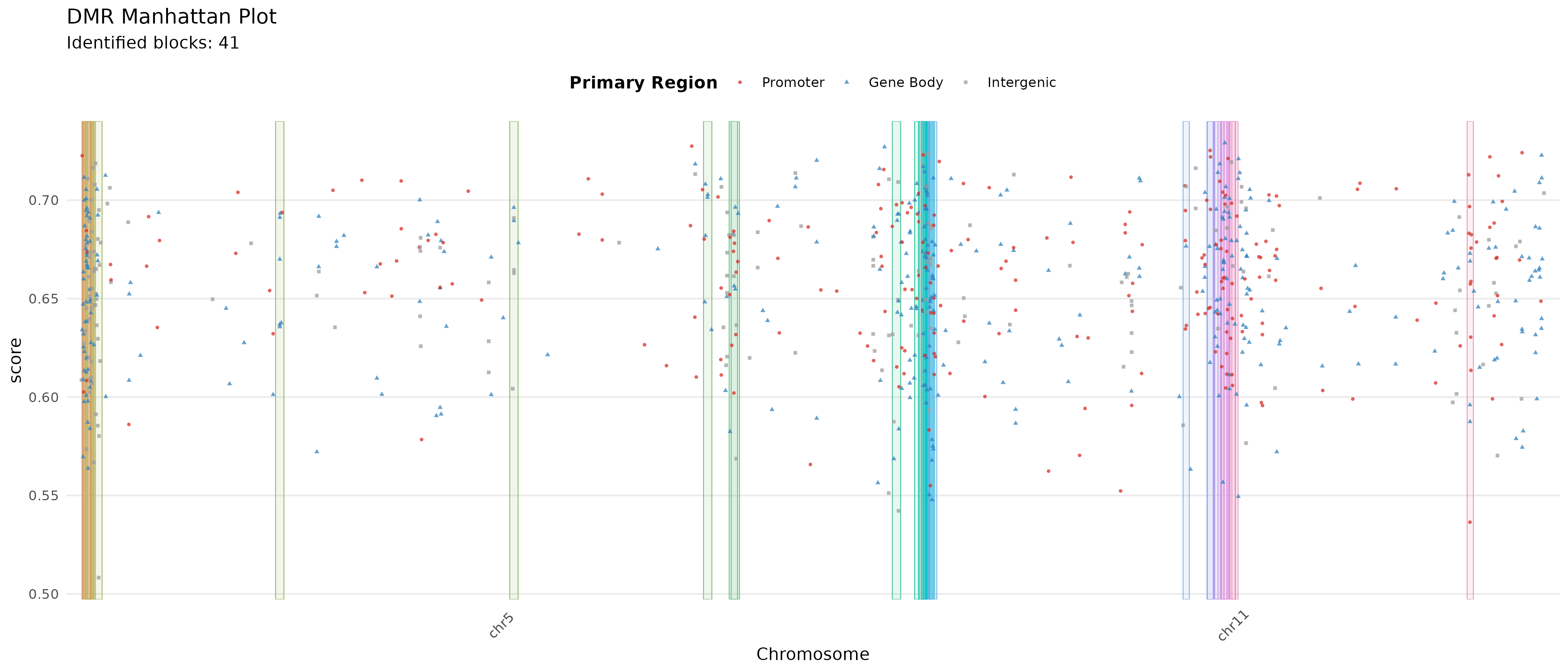
DMR Score Manhattan Plot
A manhattan plot of the DMRs is drawn, showing complementary SVM scores, their annotation as promoter or gene body DMRs, and translucent block squares for localized score peaks identified by the scoring block extension. The DMRs that belong to both promoter and gene body are omitted.
plotDMRsManhattan(
    dmrs = dmrs,
    promoter_col = "in_promoter_of",
    gene_body_col = "in_gene_body_of"
)
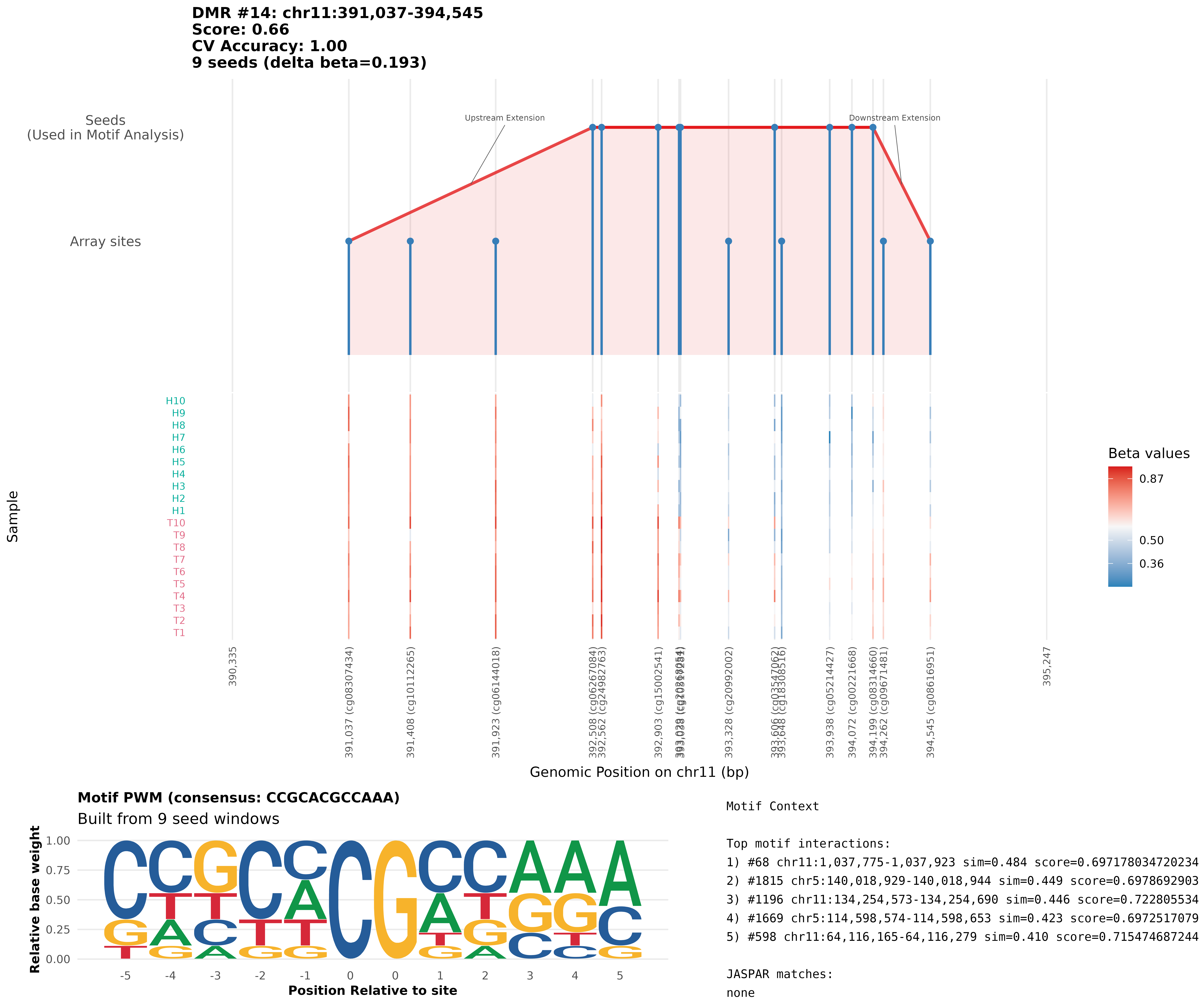
Single DMR Plot
Each DMR can be plotted with the plotDMR function, which
shows the beta values of the sites in the DMR, the seeds, and the
motif-based interactions with other DMRs, along with JASPAR annotations
if existing. Here we select a DMR that has more than one merged DMR and
has an extension beyond the seed region, in both sides.
merged_counts <- suppressWarnings(as.numeric(as.character(mcols(dmrs)$merged_dmrs_num)))
has_extension <- (mcols(dmrs)$start_seed != mcols(dmrs)$start_site) &
    (mcols(dmrs)$end_seed != mcols(dmrs)$end_site)

complex_candidates <- which(is.finite(merged_counts) & merged_counts > 1 & has_extension)
if (length(complex_candidates) == 0) {
    complex_candidates <- which(has_extension)
}
if (length(complex_candidates) == 0) {
    complex_candidates <- 1L
}

selected_dmr_idx <- complex_candidates[1]
cat(
    sprintf(
        "Selected DMR index %d (score=%s, seeds_num=%s, sites_num=%s)\n",
        selected_dmr_idx,
        as.character(mcols(dmrs)$score[selected_dmr_idx]),
        as.character(mcols(dmrs)$seeds_num[selected_dmr_idx]),
        as.character(mcols(dmrs)$sites_num[selected_dmr_idx])
    )
)
## Selected DMR index 14 (score=0.657102738173804, seeds_num=9, sites_num=16)
plotDMR(
    dmrs = dmrs,
    dmr_index = selected_dmr_idx,
    beta = beta_handler,
    pheno = pheno,
    sample_group_col = "Sample_Group",
    genome = genome,
    array = array_type,
    motif_site_flank_size = 5
)
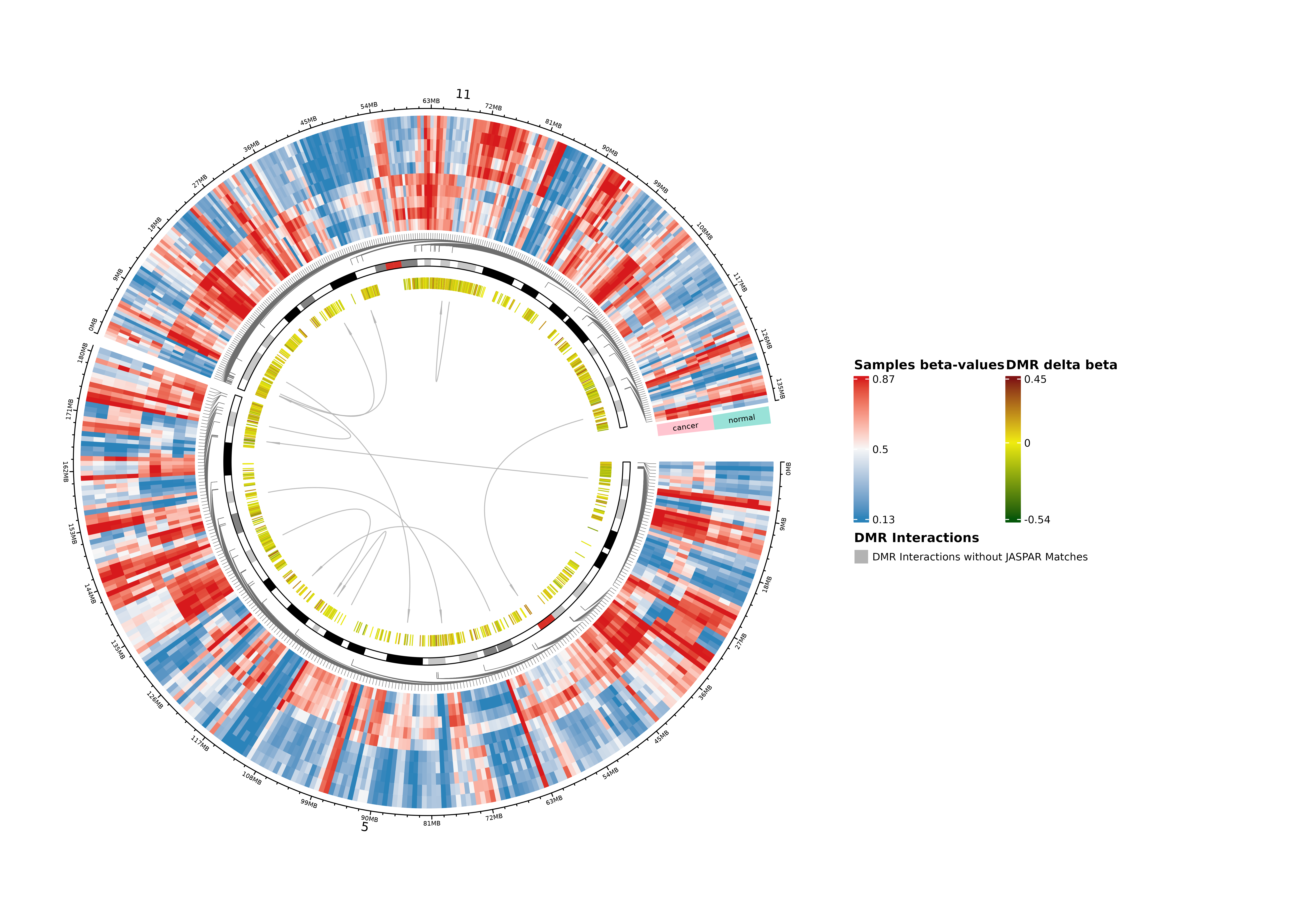
Summary Circos Plot
A circos plot consisting of the extracted information from CMEnt is drawn along the genome or a specified region. The information includes:
- The DMRs and their complementary SVM scores (at most 40 DMRs per chromosome are shown)
- Selected beta values of the DMRs (at most 5 sites per DMR, scoring by absolute delta-beta, are shown)
- The motif-based interactions between DMRs, with links direction going from higher scoring to lower scoring (at most 120 interactions groups are shown)
- The JASPAR annotation of the motif-based groups, if available, on the legend.
circos_dmrs <- dmrs
circos_summary_plotted <- FALSE

tryCatch(
    {
        plotDMRsCircos(
            dmrs = circos_dmrs,
            beta = beta_handler,
            pheno = pheno,
            genome = genome,
            array = array_type,
            sample_group_col = "Sample_Group",
            min_similarity = 0.8,
            motif_site_flank_size = 5,
            max_num_samples_per_group = 5,
            max_dmrs_per_chr = 40,
            max_sites_per_dmr = 5,
            max_components = 120,
            #region = "chr11:2Mb-5Mb, chr11:72Mb-83Mb, chr5:1Mb-12Mb", # nolint
            degenerate_resolution = 1e6,
            verbose = 1
        )
        circos_summary_plotted <- TRUE
    },
    error = function(e) {
        message("Circos plot generation failed: ", conditionMessage(e))
        NULL
    }
)
if (!circos_summary_plotted) {
    plot.new()
    text(0.5, 0.5, "Circos summary plot unavailable for this dataset.", cex = 1.1)
}
It is also possible to plot the circos for one or multiple regions to assess connectivity, e.g, for chr17:2Mb-5Mb, chr17:72Mb-83Mb and chr19:1Mb-12Mb, which are regions that in the earlier plot were shown to interact. (The reported score in the legend is computed based on the visible DMRs of each component):
circos_region_plotted <- FALSE

tryCatch(
    {
        plotDMRsCircos(
            dmrs = circos_dmrs,
            beta = beta_handler,
            pheno = pheno,
            genome = genome,
            array = array_type,
            sample_group_col = "Sample_Group",
            min_similarity = 0.8,
            motif_site_flank_size = 5,
            max_num_samples_per_group = 5,
            max_dmrs_per_chr = 40,
            max_sites_per_dmr = 5,
            max_components = 120,
            region = "chr17:2Mb-5Mb, chr17:72Mb-83Mb, chr19:1Mb-12Mb",
            degenerate_resolution = 10e2, # If the width of the DMR is larger than that, the DMRs is shown as rectangles and ribbons are used instead of links to connect the DMRs.
            verbose = 1
        )
        circos_region_plotted <- TRUE
    },
    error = function(e) {
        message("Circos plot generation failed: ", conditionMessage(e))
        NULL
    }
)
## NULL
if (!circos_region_plotted) {
    plot.new()
    text(0.5, 0.5, "Circos region plot unavailable for selected regions.", cex = 1.1)
}
CMEnt interactive Shiny App
The CMEnt interactive Shiny app can be launched with the
launchCMEntViewer function, which allows for interactive
exploration of the DMRs and the aforementioned plots. In order to use
it, the output_prefix argument should be provided in the
buildDMRs function, as the app looks for the output files
with this prefix.
launchCMEntViewer("tmp/CMEnt_example")Session Info
## R version 4.6.0 (2026-04-24)
## Platform: x86_64-pc-linux-gnu
## Running under: Ubuntu 24.04.4 LTS
##
## Matrix products: default
## BLAS:   /usr/lib/x86_64-linux-gnu/blas/libblas.so.3.12.0
## LAPACK: /usr/lib/x86_64-linux-gnu/lapack/liblapack.so.3.12.0  LAPACK version 3.12.0
##
## locale:
##  [1] LC_CTYPE=en_US.UTF-8       LC_NUMERIC=C
##  [3] LC_TIME=en_US.UTF-8        LC_COLLATE=en_US.UTF-8
##  [5] LC_MONETARY=en_US.UTF-8    LC_MESSAGES=en_US.UTF-8
##  [7] LC_PAPER=en_US.UTF-8       LC_NAME=C
##  [9] LC_ADDRESS=C               LC_TELEPHONE=C
## [11] LC_MEASUREMENT=en_US.UTF-8 LC_IDENTIFICATION=C
##
## time zone: Europe/Brussels
## tzcode source: system (glibc)
##
## attached base packages:
## [1] stats4    stats     graphics  grDevices utils     datasets  methods
## [8] base
##
## other attached packages:
##  [1] DMRsegaldata_1.0.0   ExperimentHub_3.2.0  AnnotationHub_4.2.0
##  [4] BiocFileCache_3.2.0  dbplyr_2.5.2         ggplot2_4.0.3
##  [7] GenomicRanges_1.64.0 Seqinfo_1.2.0        IRanges_2.46.0
## [10] S4Vectors_0.50.1     BiocGenerics_0.58.1  generics_0.1.4
## [13] CMEnt_0.99.0         BiocStyle_2.40.0
##
## loaded via a namespace (and not attached):
##   [1] BiocIO_1.22.0               bitops_1.0-9
##   [3] filelock_1.0.3              tibble_3.3.1
##   [5] R.oo_1.27.1                 XML_3.99-0.23
##   [7] DirichletMultinomial_1.54.0 lifecycle_1.0.5
##   [9] httr2_1.2.2                 pwalign_1.8.0
##  [11] doParallel_1.0.17           lattice_0.22-9
##  [13] backports_1.5.1             magrittr_2.0.5
##  [15] limma_3.68.4                sass_0.4.10
##  [17] rmarkdown_2.31              jquerylib_0.1.4
##  [19] yaml_2.3.12                 otel_0.2.0
##  [21] DBI_1.3.0                   RColorBrewer_1.1-3
##  [23] abind_1.4-8                 purrr_1.2.2
##  [25] R.utils_2.13.0              RCurl_1.98-1.19
##  [27] rappdirs_0.3.4              circlize_0.4.18
##  [29] seqLogo_1.78.0              testthat_3.3.2
##  [31] pkgdown_2.2.0               permute_0.9-10
##  [33] DelayedMatrixStats_1.34.0   codetools_0.2-20
##  [35] DelayedArray_0.38.2         DT_0.34.0
##  [37] tidyselect_1.2.1            shape_1.4.6.1
##  [39] futile.logger_1.4.9         ggseqlogo_0.2.2
##  [41] UCSC.utils_1.8.0            farver_2.1.2
##  [43] matrixStats_1.5.0           showtext_0.9-8
##  [45] GenomicAlignments_1.48.0    jsonlite_2.0.0
##  [47] GetoptLong_1.1.1            iterators_1.0.14
##  [49] systemfonts_1.3.2           foreach_1.5.2
##  [51] tools_4.6.0                 ragg_1.5.2
##  [53] TFMPvalue_1.0.0             Rcpp_1.1.1-1.1
##  [55] glue_1.8.1                  gridExtra_2.3
##  [57] SparseArray_1.12.2          xfun_0.58
##  [59] MatrixGenerics_1.24.0       GenomeInfoDb_1.48.0
##  [61] dplyr_1.2.1                 HDF5Array_1.40.0
##  [63] withr_3.0.2                 formatR_1.14
##  [65] BiocManager_1.30.27         fastmap_1.2.0
##  [67] bedr_1.1.5                  rhdf5filters_1.24.0
##  [69] caTools_1.18.3              digest_0.6.39
##  [71] R6_2.6.1                    textshaping_1.0.5
##  [73] colorspace_2.1-2            gtools_3.9.5
##  [75] dichromat_2.0-0.1           RSQLite_3.53.1
##  [77] cigarillo_1.2.0             R.methodsS3_1.8.2
##  [79] h5mread_1.4.0               data.table_1.18.4
##  [81] rtracklayer_1.72.0          FNN_1.1.4.1
##  [83] httr_1.4.8                  htmlwidgets_1.6.4
##  [85] S4Arrays_1.12.0             TFBSTools_1.50.0
##  [87] pkgconfig_2.0.3             gtable_0.3.6
##  [89] blob_1.3.0                  ComplexHeatmap_2.28.0
##  [91] S7_0.2.2                    XVector_0.52.0
##  [93] brio_1.1.5                  htmltools_0.5.9
##  [95] sysfonts_0.8.9              bookdown_0.46
##  [97] strex_2.0.1                 clue_0.3-68
##  [99] scales_1.4.0                Biobase_2.72.0
## [101] png_0.1-9                   knitr_1.51
## [103] lambda.r_1.2.4              reshape2_1.4.5
## [105] rjson_0.2.23                checkmate_2.3.4
## [107] curl_7.1.0                  showtextdb_3.0
## [109] cachem_1.1.0                rhdf5_2.56.0
## [111] GlobalOptions_0.1.4         stringr_1.6.0
## [113] BiocVersion_3.23.1          parallel_4.6.0
## [115] AnnotationDbi_1.74.0        restfulr_0.0.16
## [117] desc_1.4.3                  pillar_1.11.1
## [119] grid_4.6.0                  vctrs_0.7.3
## [121] beachmat_2.28.0             cluster_2.1.8.2
## [123] JASPAR2024_0.99.7           evaluate_1.0.5
## [125] bsseq_1.48.0                VennDiagram_1.8.2
## [127] cli_3.6.6                   locfit_1.5-9.12
## [129] compiler_4.6.0              futile.options_1.0.1
## [131] Rsamtools_2.28.0            rlang_1.2.0
## [133] crayon_1.5.3                labeling_0.4.3
## [135] plyr_1.8.9                  fs_2.1.0
## [137] stringi_1.8.7               gridBase_0.4-7
## [139] BiocParallel_1.46.0         Biostrings_2.80.1
## [141] Matrix_1.7-5                BSgenome_1.80.0
## [143] sparseMatrixStats_1.24.0    bit64_4.8.2
## [145] Rhdf5lib_2.0.0              KEGGREST_1.52.0
## [147] statmod_1.5.2               SummarizedExperiment_1.42.0
## [149] igraph_2.3.2                memoise_2.0.1
## [151] bslib_0.11.0                bit_4.6.0